BackTest on ARIMA Forecast in Python

ARIMA is one of the most essential time-series-estimation methods. In this article, I am going through its basic and crucial elements, including tests of stationary and white noise before ARIMA modeling and predicting.

The results only include estimation of price, and backtest results like Sharpe are not calculated.

Firstly, we are doing some data preprocessing. The data 'SH50 Price.csv' includes the price information of the 50 listed in Shanghai Stock Exchange, components of SSE50 index, from 2009 to 2013. Data is available here.

# Data Preprocessing
import math
import pandas as pd
import numpy as np
from matplotlib import pyplot as plt
import ffn
df = pd.read_csv('SH50 Price.csv')
df.Date = pd.to_datetime(df.Date)
stocks = df.columns[1:].tolist()
prices = df[stocks]
prices.index = df.Date
simret = ffn.to_returns(df[stocks])
simret.index = df.Date
p_stk = prices['Stk_600000'][1:]
r_stk = simret['Stk_600000'][1:]

After preprocessing, we obtain price series 'p_stk' and returns series 'r_stk'. Then, we are going to have a glance at the information provided in the datasets. We choose stk 600000 as our target to research and forecast.

# Part I: Print figures
plt.figure(dpi=200)
plt.plot(p_stk)
plt.title('Price of Stk 600000')
plt.savefig('Price of Stk 600000.png')
plt.figure(dpi=200)
plt.plot(r_stk)
plt.title('Returns of Stk 600000')
plt.savefig('Returns of Stk 600000.png')

The plots are:

Because ARIMA requires that the time series should be stationary and not white noise, in the following two parts, we are using ADF Unitroot Test and Ljung-Box White Noise Test to evaluate the characteristics of the price and returns series.

# Part II: Test Stationary: ADF unitroot test
from arch.unitroot import ADF
adf = ADF(p_stk)
print(adf.summary()) #p-value: 0.042
adf = ADF(r_stk)
print(adf.summary()) #p-value: 0.000

Both of them are stationary, while returns series are more stationary as it has significantly smaller p-value, even though the p-value of prices are lower than 5%.

# Part III: Test White Noise: Ljung-Box test
from statsmodels.tsa import stattools
LjungBox_p = stattools.q_stat(stattools.acf(p_stk)[1:12],len(p_stk))
LjungBox_r = stattools.q_stat(stattools.acf(r_stk)[1:12],len(r_stk))

>> LjungBox_p
(array([  1186.72403401,   2347.64336586,   3480.90920079,   4585.93740601,
          5664.13867134,   6714.87739681,   7742.00626975,   8745.83186807,
          9727.36536476,  10686.98822401,  11624.15953127,  12540.96124026,
         13436.9868527 ,  14312.56022102,  15168.03444284,  16003.30196641,
         16817.86975455,  17612.10904286,  18385.5534396 ,  19138.93560575,
         19870.54594297,  20580.38199531,  21268.22774876]),
 array([  4.68328128e-260,   0.00000000e+000,   0.00000000e+000,
          0.00000000e+000,   0.00000000e+000,   0.00000000e+000,
          0.00000000e+000,   0.00000000e+000,   0.00000000e+000,
          0.00000000e+000,   0.00000000e+000,   0.00000000e+000,
          0.00000000e+000,   0.00000000e+000,   0.00000000e+000,
          0.00000000e+000,   0.00000000e+000,   0.00000000e+000,
          0.00000000e+000,   0.00000000e+000,   0.00000000e+000,
          0.00000000e+000,   0.00000000e+000]))

>> LjungBox_r
(array([  5.74442324e-05,   6.94963524e-01,   2.36008649e+00,
          2.56248994e+00,   3.34789797e+00,   8.93787714e+00,
          9.12876556e+00,   9.22065050e+00,   9.59020002e+00,
          9.72752825e+00,   1.23203023e+01,   1.34820767e+01,
          1.38328148e+01,   1.41616503e+01,   1.41655260e+01,
          1.61315152e+01,   1.61315159e+01,   1.76274610e+01,
          1.78485936e+01,   2.20053144e+01,   2.20102166e+01,
          2.20334465e+01,   2.20547776e+01]),
 array([ 0.99395273,  0.7064649 ,  0.50110775,  0.63348204,  0.64651689,
         0.17710208,  0.24354298,  0.32402559,  0.38466708,  0.46471465,
         0.340055  ,  0.3349957 ,  0.38572255,  0.43773873,  0.51301413,
         0.44382027,  0.51453146,  0.48043601,  0.5325723 ,  0.34022234,
         0.39892134,  0.45789384,  0.5169469 ]))

The null hypothesis is the series is white noise, and when the p-values (lower part of the result) of corresponding scores (upper part) are very small, we would reject the null hypothesis. In the prices, all values are highly significant, while the returns cannot reject the hypothesis (with 24 lags, the lowest one is even more then 10%).

Therefore, we accept that returns series are white noise, and we would only use price series in the following analysis.

# Part IV: Determine the order p and q in ARMA(p,q)

In part IV, we will use ARMA instead of ARIMA because we have already determined that order of I, d = 0 because returns are white noise. Next, we will determine the orders of ARMA(p,q).

Our first method to determine orders:

Draw ACF and PACF, and we found that ACF decays slowly while PACF suddenly drops, indicating an AR process only. We calculate its corresponding AIC and fit them with AR, setting maximum number of lags to be 12, and get the result that 1 is great. Check again with PACF plot, only lag 1 has significant coefficient. Therefore, we determine it to be AR(1) process.

from statsmodels.graphics.tsaplots import plot_acf, plot_pacf
axe1 = plt.subplot(211)
axe2 = plt.subplot(212)
plot1 = plot_acf(p_stk,lags=24,ax=axe1)
plot2 = plot_pacf(p_stk,lags=24,ax=axe2)
# Clear trend of AR only, with order for MA q = 0
# According to PACF, order p = 1
from statsmodels.tsa import ar_model
print(ar_model.AR(p_stk).select_order(maxlag=12,ic='aic')) # 1

Our alternative method to determine orders: Calculate the information criteria values of each order pairs.

order_determine = stattools.arma_order_select_ic(p_stk,ic=['bic','aic'])

>>order_determine
{'aic':              0            1            2
 0  9463.164218  8000.817909  7042.006694
 1  4518.521655  4520.130771  4520.321662
 2  4520.100423  4520.516399  4521.249129
 3  4520.254865  4521.373563          NaN
 4  4520.303277  4520.282986  4517.939588,
 'aic_min_order': (4, 2),
 'bic':              0            1            2
 0  9473.360970  8016.113036  7062.400197
 1  4533.816782  4540.524274  4545.813540
 2  4540.493925  4546.008277  4551.839383
 3  4545.746743  4551.963817          NaN
 4  4550.893531  4555.971616  4558.726593,
 'bic_min_order': (1, 0)}

As BIC is more robust, the AIC of (1,0) is enarly the same with (4,2), and lower orders are better models to avoid overfitting risk, we choose ARMA(1,0), which leads to the same results with the above method.

# Part V: Fit prices with ARIMA(1,0,0) (Also ARMA(1,0) or AR(1))
# from statsmodels.tsa import ar_model
model = ar_model.AR(p_stk).fit(maxlag=12,method='cmle',ic='aic')
# arima_model package is a similar package, leading to a same result
from statsmodels.tsa import arima_model
model2 = arima_model.ARIMA(p_stk,order=(1,0,0)).fit()

Even though 'model' is the same with 'model2', the package ar_model has some bugs as I test it, and the package arima_model has attribute 'forecast' and it is more convenient to use this one. So, we only use model2 in the following parts.

>>model2.summary()

After ARMA modeling, we need to test whether the results of ARMA is white noise. If not, we may need more thorough researches. Fortunately, the results in the following shows that our result is white noise and no auto-correlation patterns.

# Part VI: Robustness Check: Test on Residuals
res = model2.resid
stdres = res/math.sqrt(model2.sigma2)
plt.figure(dpi=200)
ax1 = plt.subplot(211)
ax2 = plt.subplot(212)
ax1.set_title('standard residuals')
ax1.plot(stdres)
plot_acf(stdres,lags=24,ax=ax2)
plt.savefig('test_on_residuals_of_ARMA.png')

# Ljung-Box White Noise tests:
LjungBox_m = stattools.q_stat(stattools.acf(stdres[1:])[1:24],len(stdres[1:]))
# Residuals are White Noises
>>LjungBox_m
(array([  0.27569431,   1.76892747,   3.40736876,   4.00228122,
          4.30689222,   8.74894778,   8.75161177,   8.79754988,
          8.84251288,   9.8780216 ,  12.49860582,  13.03671273,
         13.05266838,  13.31819495,  13.83520634,  16.51855888,
         16.83245856,  18.33579538,  18.40466682,  23.02723339,
         23.05146308,  23.051464  ,  23.17217018]),
 array([ 0.59953731,  0.41293556,  0.33297629,  0.40569721,  0.50612843,
         0.18819711,  0.27098469,  0.35966135,  0.45193696,  0.45125936,
         0.32735392,  0.3663779 ,  0.44375169,  0.50163586,  0.53806246,
         0.41739165,  0.46577191,  0.43374623,  0.49557738,  0.2874593 ,
         0.34124064,  0.39882846,  0.45075531]))

To conclude, we cannot reject that results white noise, and the ARMA models can be used to forecast.

In the next part, we are going to give a forward forecast on the results, and plot corresponding confidence intervals.

# Part VII: Forecast
forecast = model2.forecast(steps=15)
plt.figure(dpi=200)
plt.grid(True)
plt.xticks(rotation=15)
plt.title('ARIMA(1,0,0) Forecast for Stk 600000')
plt.plot(p_stk[-30:])
dates = pd.DatetimeIndex(freq='d',start='2014-01-01',end='2014-01-15')
plt.plot(dates,forecast[0])
plt.plot(dates,forecast[2][:,0],ls=':')
plt.plot(dates,forecast[2][:,1],ls=':')
plt.legend(['real','pred','lc','uc'])
plt.savefig('ARIMA_forecast.png')

Finally, we perform out-of-sample test of ARIMA(1,0,0) by estimating one-day-forward price in each day of the sets with models built by the previous data. Continue the test every day beginning in the 100th index, and calculate the results. Because of limited space, we only provide a plot including the last 110 sets of predicted price against real price.

# Part VIII: Out-of-Sample Test for ARIMA(1,0,0) Performance
preds = []; lcs = []; ucs = []
for i in range(100,len(p_stk)):
    model_o = arima_model.ARIMA(p_stk[:i],order=(1,0,0)).fit()
    preds.append(model_o.forecast(1)[0][0])
    lcs.append(model_o.forecast(1)[2][0][0])
    ucs.append(model_o.forecast(1)[2][0][1])
plt.figure(dpi=200)
plt.grid(True)
plt.xticks(rotation=15)
plt.title('Real against One-Day-Forward-Forecast')
plt.plot(p_stk[1000:],ls='-')
dates = p_stk.index[1000:]
plt.plot(dates,preds[900:],lw=0.5)
plt.legend(['real','pred_ar1'])
plt.savefig('ARIMA_OStest.png')

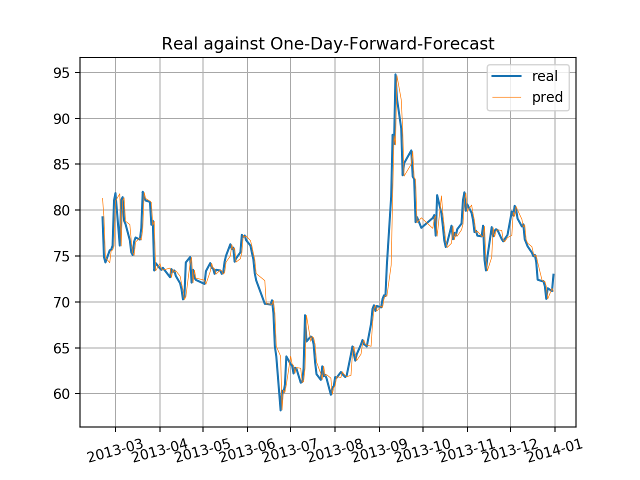
By the way, we plot the errors of real minus estimated, and the result is very similar with the shape of returns. The errors might have patterns of heteroscedasticity, and perhaps one way to improve is to introduce ARCH or GARCH.

errors = p_stk[100:] - pd.Series(preds,index=p_stk.index[100:])
plt.figure(dpi=200)
plt.title('Errors of ARMA OS test')
plt.plot(errors)
plt.savefig('errors_of_ARIMA_OStest.png')

Reference:
Quantitative Investment Using Python, written by Lirui CAI, a Chinese Book named《量化投资：以Python为工具》

Feasible GLS (Generalized Least Squares)

GLS is applied when the residuals of OLS cannot satisfy two aspects of its classical assumptions: homoscedasticity and no auto-correlation, or rather,

$E(uu^{'})=\sigma ^{2}\Omega $

rather than

$E(uu^{'})=\sigma ^{2}I$

There are many forms of FGLS, and the following passage describes its basic theorem and one form of FGLS that could eliminate if there is only heteroscedasticity:

Theorem of GLS, WLS, and One Form of FGLS

There is also another model to eliminate only AR(1) pattern in the OLS residuals:

1) Estimate coefficient $\rho$ in the residuals that

$e_{t} = \rho e_{t-1} + \varepsilon$

2) Transfer

$y = X\beta +u $

to

$Py = PX\beta +Pu $

by

and 3) Estimate correspondingwith OLS estimation.

I will add more forms of FGLS in the following if possible.

Articles Related with Options Trading Strategies: Reading List

On Feb. 2018:

I.

Dubinsky A, Johannes M. Fundamental uncertainty, earning announcements and equity options[R]. Working paper, 2006.

Abstract:

This paper uses option prices to learn about the uncertainty surrounding the fundamental information that is revealed on earnings announcement dates. To do this, we introduce a reduced-form model and estimators to separate the uncertainty over the information revealed on earnings dates from normal day-to-day volatility. The fundamental uncertainty estimators are easy to compute and rely only on option price information available prior to the announcement. Empirically, we find strong support for our reduced form specification and investigate the fundamental uncertainty estimators. We find that they are quantitatively large, vary over time, and are informative about the future volatility of stock price movements. Finally, we quantify the impact of earnings announcements on formal option pricing models.

II.

Xing Y, Zhang X. Anticipating uncertainty: Straddles around earnings announcements[J]. 2013.

Abstract:

Straddles on individual stocks generally earn significantly negative returns. However, average at-the-money straddles from three days before an earnings announcement to the announcement date yield a highly significant 3.34% return. The positive returns on straddles indicate that investors under-estimate the magnitude of uncertainty around earnings announcements. We find positive straddle returns are more pronounced for smaller firms, firms with higher volatility, higher kurtosis, more volatile past earnings surprises and less trading volume/higher transaction costs. This
suggests that when firm signals are noisy, and/or when it is costlier to trade, investors underestimate the uncertainty associated with earnings announcements.

III.

Cremers M, Fodor A, Weinbaum D. How Do Informed Option Traders Trade? Option Trading Activity, News Releases, and Stock Return Predictability[J]. 2017.

Abstract:

We examine how informed traders trade in the option market around news announcements. Option traders are more active, and their trades more informative, both immediately before news days and on news days. How informed option traders implement their trades depends on when they trade and whether news releases are scheduled: we predict and find that informed option traders use short positions (instead of long positions) before scheduled news announcements. Purchases of options thus predict returns on news days and ahead of unscheduled events, but not before scheduled events, and sales of options are informative only ahead of scheduled news releases.

IV.

Jones C S, Shemesh J. Option Mispricing Around Nontrading Periods[J]. The Journal of Finance, 2017.

Abstract:

We find that option returns are significantly lower over nontrading periods, the vast majority of which are weekends. Our evidence suggests that nontrading returns cannot be explained by risk, but rather are the result of widespread and highly persistent option mispricing driven by the incorrect treatment of stock return variance during periods of market closure. The size of the effect implies that the broad spectrum of finance research involving option prices should account for nontrading effects. Our study further suggests how alternative industry practices could improve the efficiency of option markets in a meaningful way.

BackTest on Displaced Moving Average (DMA): Simple is Good!

Displaced Moving Average, is perhaps one of the most simple technical indexes that I have ever tested, but it is one of the most stable technical indexes that I have ever seen among different Futures Contracts.

I tested it against all the contracts listed in China Futures Market, and it turned out that most of them suit pretty well. In daily basis, DMA is strong enough to capture big trends in price movements.

Let's look at the definition and formula of it:

Components:

• MA(t,12) = Simple Moving Average for close price in 12 days
• MA(t,26) = Simple Moving Average for close price in 26 days
• DMA(t) = MA(t,12) - MA(t,26)
• AMA(t,9) = Simple Moving Average for DMA in 9 days

Strategy:

• Long on the spot that DMA surpasses AMA
• (DMA(t) > AMA(t) and DMA(t-1) <= AMA(t-1))
• Short on the spot that DMA surpassed by AMA
• (DMA(t) < AMA(t) and DMA(t-1) >= AMA(t-1))

Even though, the results of DMA is vulnerable to different Futures Contract, but the truth is, when we combine them together, then the outcome is beautiful.

* Click this link to check out the performance of each individual Futures Contract:

https://drive.google.com/open?id=19DnrN0YQlJkcelnBzm4M6YAoE345p-4F

Profits & Loss of the entire Market:

The Sharpe of it, is 1.33, which is already very good as daily trend capturing strategies are not that stable, and this Sharpe suggests the stability of the entire strategy.

Note that cash, accounts, and trading volumes have not been adjusted for different kinds of Futures Contracts, and we assume that the maximum holding positions for all of them are 3 volume, and therefore the profit or loss from each individual contracts may be different.

But generally speaking, the results are stable even for the fact that individual risk has not been eliminated, as we can simply deduct the most profitable and least profitable contracts as follow:

We can observe that even though the absolute value of profits have been changed, the shape of it is stable. This partly suggest that our belief that DMA is stable in different contracts is reasonable.

Considering the fact that how simple DMA is, many of us assume that such index is no longer effective, and it is debatable whether the market is efficient and technical analysis is useless.

So, it can be possible the entire performance is out of luck. Therefore, be careful when investing with technical analysis.

* Source Code and Raw Data are not applicable.

On Sharpe Ratio: The Higher, The Better?

Sharpe Ratio is perhaps one of the most famous and powerful ways to evaluate the performance of a portfolio.

$Sharpe\ Ratio = \frac{Risk\ Premium}{SD\ of\ excess\ return}$

In most cases, Sharpe Ratio is used as a quick way to reflect the reward to volatility of a portfolio:

The higher Sharpe Ratio is, the more risk premium we assume that is coming from a given "volatility".

For example, some big trading companies may categorize funds with Sharpe more than 2 as spectacular, more than 1.5 as excellent, more than 1.25 as good, more than 1 as average, less than 1 as inferior...

HOWEVER, given different time horizons of a portfolio, while others remain constant, Sharpe can be completely different, and evaluation based merely on Sharpe can be misleading.

To understand this, let's first dive into the components of Sharpe Ratio:

I. Risk Premium

To begin with, assume we have all the data of monthly return of Baidu. We fear that there may be some scandals tomorrow and influence its cash flow in the future, and in the meanwhile we also hope a new version of auto-mobile car invented in the next month.

To bear this kind of risk, a risk-averse investor (we assume all the investors are risk-averse) would then expect a higher return in the future.

But how to estimate excess return? The most widely-used way is to use the arithmetic average return minus risk-free rate as the estimation of risk premium.

$\widehat{E(r)}=\frac{1}{n}\sum_{i=1}^{n} r_i$

Under the assumption of normal return distribution, the above estimation is unbiased.

Expected Return minus Risk-free Rate, and we can get our unbiased estimation of Risk Premium.

II. Volatility: Standard Deviation of Excess Return

A generally accepted valuation of expected volatility is standard deviation $\sigma $.

Some claim that we care only about the downward risk. However, Bodie argued that as long as the probability distribution is more or less symmetric about the mean, $\sigma $ is a reasonable measure of risk.

$\widehat{E(\sigma ^2)}=\frac{1}{n-1}\sum_{i=1}^{n} (r_i-\bar{r})^2$

Under normal assumption, such estimation of standard deviation is unbiased as the degrees of freedom bias is eliminated.

III. Time Horizons: a variable greatly easy to be ignored

Now, we already have the estimations of Risk Premium as well as Estimated Volatility, and simply divide them, we can derive Sharpe Ratio.

What seems to be the problem?

Given monthly average excess return r, and monthly standard deviation $\sigma$, assume that returns among each month is i.i.d., and annually estimated excess return is $12r$, while annually estimated standard deviation is $\sqrt{12}\sigma$

Therefore, now the annual Sharpe Ratio is $\sqrt{12}\frac{r}{\sigma}$, while the monthly Sharpe Ratio is $\frac{r}{\sigma}$.

This indicates that a same portfolio can be measured with drastically different Sharpe Ratio!

For example, if the previous annual Sharpe Ratio is 1.50, labeled as excellent previously, would soon become 0.43, which is inferior in a monthly basis.

However, in practice, we merely mention that "My Sharpe is 2 in an annual basis", but "The Sharpe of my strategy is 2".

We simply ignore one factor that may change the entire story.

BackTest on MACD, KDJ, and RSI

MACD, KDJ, and RSI are three powerful technical indices. These indices are widely used to reflect trend, especially reversal trend.

Simply speaking, when one of these indices is triggered, then:

• An upward trend may reverse to a downward trend, OR,
• A downward trend may reverse to an upward trend

The performance of those indices are more or less affected by the extraneous parameters (like the x in "highest price in x days"), but here we assume all of these parameters set to be generally accepted parameters.

To specify, here we assume that:

MACD:

Estimation Formula:

• EMAS(t) = Exponential Moving Average of Price in Short Term (daily close price in 12 days)
• EMAL(t) = Exponential Moving Average of Price in Long Term (daily close price 26 days)
• DIF(t) = EMAS(t) - EMAL(t)
• DEA(t) = Exponential Moving Average of DIF (in 9 days)
• MACD(t) = [DIF(t) - DEA(t)] * 2

Strategy:

• Long when MACD is negative and increasing
• Short when MACD is positive and decreasing

KDJ:

Estimation Formula:

• Low(t,9) = Lowest price in 9 days (date t-9 to t)
• High(t,9) = Highest price in 9 days (date t-9 to t)
• RSV(t) = (Close(t) - Low(t,9)) / (High(t,9) - Low(t,9))
• K(t) = RSV(t)/3 + 2*K(t-1)/3
• D(t) = K(t)/3 + 2*D(t-1)/3
• J(t) = 3*K(t) - 2*D(t)

Strategy:

• Long when J is <= 25 and increasing
• Short when J is >= 75 and decreasing

RSI:

Estimation Formula:

• MEANUP(t,12) = Mean of positive returns in the last 12 days
• MEANDOWN(t,12) = Absolute value of the Mean of negative returns in the last 12 days
• RS(t) = MEANUP(t,12)/MEANDOWN(t,12)
• RSI(t) = 100 - 100 / [ 1+ RS(t) ]

Strategy:

• Long when RSI is <= 40 and increasing
• Short when RSI is >= 60 and decreasing

Backtest Results:

Ag: Silver/ Agrentum Futures, listed on Shanghai Futures Exchange, China

Profits & Loss:

MACD:

KDJ: 

RSI:

However, there is one BIG problem.

All of these indices, are highly sensitive to different underlying assets. Those performance that is beautiful in Ag, might be pretty bad in some others.

In fact, I have also tested all the other active 34 Futures Contracts listed in China (see in *1), and none of them performs similarly to Ag. Some of the three strategies are valid for some of them, while others may not:

It is possible that good results come from pure luck, not the effectiveness of strategy itself.

Therefore, single index should never be considered the sole best strategy. Like Alpha seeking, a better strategy may be effective when more financial instruments are taken into account.

By the way, one another thing may help: decrease the cycle of investments:

For example, in these examples (MACD/KDJ/RSI), all prices are updated upon daily basis. However, investing in such a long term is more like a fundamental analysis, which is basically too risky to quantitative investments: the max drawdown may be very drastic.

But, can we really transform it into smaller cycles?

I have changed my updating criteria, from daily to every 5 minute of market-time, and all the other variables remain the same.

For instance:

• The highest price in 9 days now refers to the highest price in 9 5-minute-time, i.e., 45 minutes

Let's see the results:

Profits & Loss:

MACD:

KDJ:

RSI:

Surprise! (In fact, not very surprise to professionals)

A beautiful smooth downward curve! It strongly supports the idea that if we keep the status quo, then all the trends captured by daily cycle would soon disappear in a 5-minute cycle.

Therefore, in determining smaller cycles, we need to be more careful.

I will do some smaller cycle analysis and combining singular trend capturing strategies in the next time.

* 1 See the performance of all the other active Futures Contracts at:
https://drive.google.com/open?id=1V1GF93pYCEmxnfwPCxeOvzqCaUE8ilzU

* 2 For some reasons, Source Code and raw data is not applicable.

* 3 I have tested the precision of MACD, RSI and KDJ prediction of the trend tomorrow. They are mostly around 45%-48%. This seems to be very frustrating but the reality is the correct trend these indexes have captured can be those drastic trend and once captured successfully a large amount of profits can be realized.

BackTest on Dual Thrust

Dual Thrust is basically one of the first investment strategies that I have developed and tested.

It was developed by Michael Chalek in 1980s, and it was one of the most profitable strategies at that time.

Its general idea is to capture an upward or downward momentum signaled by a suddenly increased or decreased price.

This strategy is determined by two lines: one buy-line, the other one sell-line. If the close price / current price is higher than the buy-line, then buy one; else if lower than sell-line, then sell one.

Buy/Sell-line is based on the volatility of current price. Specifically, it is the open price of a certain date plus or minus the parameter 'k' times an another parameter 'range'. Range is composed of max(Highest_High - Lowest_Close, Highest_Close - Lowest_Low), which can be shown more clearly in the followings.

In expression:

• HH = highest highest price in n days 
• HC = highest close price in n days
• LC = lowest close price in n days
• LL = lowest lowest price in n days
• range = max(HH-LC, HC-LL)
• buyline = open + k1*range
• sellline = open - k2*range

Here we assume that

• Parameter date is n
• k1 = k2 = K

The performance of this strategy is doubted. But, why still using such an old, out of date strategy?

For one, I am a Chinese market potential investor. Though it has been generally accepted that US markets are already weakly efficient, Chinese financial markets are still far from that.

For another, Dual Thrust is easy to understand and simple to test.

The financial market I will be testing is Shanghai Futures Exchange, China, and the financial instrument is Futures contracts of Aluminum.

All the data were selected from CSMAR on a daily basis (国泰安金融数据库).


The result is:

Continue with sensitive analysis: change parameters K and date, and we have:

Sharpe       K = 0.5     K = 0.7
date = 8       1.36          1.40
date = 12     1.63         -0.09
date = 16     1.60          1.45

To conclude, we have:

Advantages:

• Easy to understand and implement

Disadvantages:

• Static strategies, needs dynamical parameter adaptation
• Parameters like K and date are sensitive to changes
• No underlying theory about the authenticity of each parameter

Potential improvements:

• Smaller trends (e.g. 5-minute Candlestick chart) may stabilize profits in a shorter-run
• Adjust parameters based on volatility

Conclusion:

• Static traditional Dual Thrust is valid but not very strong. Its performance is sensitive to many factors, and to improve the performance many improvements need to be done.

Source Code File: To be updated
Raw Data: To be updated