Saturday, March 24, 2018

Mind-Map for Junior Students Looking for Quantitative Research Positions

This roadmap is what I thought that should be beneficial for students like me who are interested in a quantitative research position in financial institutions, especially in hedge funds.

In my opinion, Finance, Mathematics, Statistics, Computer Science and Soft Skills are key elements to successfully looking for such a job. Sadly, the red blanks showed what I have not learnt yet, and not having basic knowledge in these fields might prevent me from having a competitive competence.

Hopefully, this graph could remind me of what is important for my career and what is not, and it should be much better if it could be beneficial for others who are also highly interested in quant research.

Image:


Friday, March 9, 2018

Black-Scholes Option Pricing Model and Empirical Analysis on 50ETF Option

In the previous blog, I tried Binomial-Tree Model to price 50ETF option in China, where I found it significantly underestimated the price. In the following analysis, I choose Black-Scholes Model instead, but found that although the difference of the predicted prices are significantly different with a p-value around 0.03, the results of prediction is pretty similar, leading to the same conclusion: Black-Scholes Model also underestimates the price of 50ETF option in China.

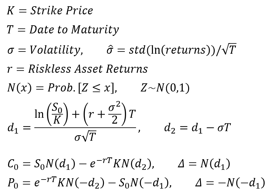
The formula of Black-Scholes is as follow:


I have also written the codes of estimating prices under BS Model:

from scipy import stats
def Black_Scholes(r,sig,S0,K,T,isCall):
    # European Option Pricing
    d1 = (np.log(S0/K) + (r+sig**2/2)*T)/(sig*np.sqrt(T))
    d2 = d1 - sig*np.sqrt(T)
    if isCall == True:
        C0 = S0*stats.norm.cdf(d1,0,1)-np.exp(-r*T)*K*stats.norm.cdf(d2,0,1)
        return C0, stats.norm.cdf(d1,0,1)
    else:
        P0 = -S0*stats.norm.cdf(-d1,0,1)+np.exp(-r*T)*K*stats.norm.cdf(-d2,0,1)
        return P0, -stats.norm.cdf(-d1,0,1)

Keep all the other methods the same with the previous blog, only replace the function to price option under binomial-tree model with the function above, and increase the test period from the range of (2015-07-31, 2015-11-30) to (2015-07-31, 2016-03-22), the results of the prices are stored in this file: binomialResults_Binomial&BS.csv

Visualizing the difference between the two models, and we find that these two models nearly predict the same results:

plt.figure(dpi=200)
plt.title('Binomial Against Black-Scholes Price')
plt.xlabel('Binomial Price')
plt.ylabel('Black-Scholes Price')
plt.xlim(0,0.6); plt.ylim(0,0.6)
plt.plot(df_results.BinomialPrice,df_results.BSPrice,ls=' ',marker='.')
plt.savefig('Binomial Against Black-Scholes Price.png')


Although statistical analysis (t-test on the differences) shows that the results are significantly different with a p-value of around 0.03:

diff = df_results.BinomialPrice-df_results.BSPrice
ttest_1sample = stats.ttest_1samp(diff, 0)

In [1]: ttest_1sample
Out[1]: Ttest_1sampResult(statistic=2.1480372929383886, pvalue=0.031870221099299899)

Then we may conclude that although slightly different, Binomial-Tree and Black-Scholes Models predict nearly the same prices on 50ETF option from 2015-07-31 to 2016-03-22. Plot Black-Scholes Price against Real Price, and we can find it also significantly underestimates the price of options.

plt.figure(dpi=200)
plt.title('Black-Scholes Price against Real Price')
plt.xlabel('Black-Scholes Price')
plt.ylabel('Real Price')
plt.xlim(0,0.6); plt.ylim(0,0.6)
plt.plot(df_results.BinomialPrice,df_results.Close,ls=' ',marker='.')
plt.savefig('Black-Scholes Price against Real Price.png')


Binomial-Tree Option Pricing Model and Empirical Analysis on 50ETF Option

I have implemented binomial-tree option pricing model to the only listed financial option in China: option on 50ETF. The results show that though somewhat similar, binomial-tree model cannot successfully price the options, and it might underestimate the risks which could lead to raising the prices.

I. Basic Steps on Binomial-Tree Model

Binomial-Tree Model assumes that in each time period, the stock price would either go up or go down, with a similar scale, as shown in the following graph:


Assuming that we know the exact parameter of the growth and the variance, we can calculate the expected tree of stocks. Specify a certain dt up to its exercise date, we may get a stock tree.


After building the stock tree, we can derive the corresponding option tree. However, unlike calculating from the first node, in the Binomial-Tree Model, we calculate the price of the option from the end of the tree. That is, we calculate all the possible prices of option on the exercise date, and backwardly propagating the previous prices by the formula shown above, and leading to the estimated price at present.

We can also calculate the delta by (C(1,1)-C(1,0))/(S(1,1)-S(1,0)) to show the sensitivity of option to its underlying asset.

Similarly, replacing C(N,m) = Max(S(N,m)-K,0) with Max(K-S(N,m),0), we can derive the price at exercise date of the put option, and by remaining other steps the same, we might calculate the P(0,0) and its delta.

The Python codes of binomial tree are shown as following:

import numpy as np
def binomial_tree(r,mu,sig,S0,K,T,N,isCall):
    # European Option Pricing
    dt = T/N
    q=(np.exp(r*dt)-1-mu*dt)/(2*sig*np.sqrt(dt))+0.5;
    U=1+mu*dt+sig*np.sqrt(dt)
    D=1+mu*dt-sig*np.sqrt(dt)
    DCF=np.exp(-r*dt)
    S=np.zeros((N+1,N+1))
    C=np.zeros((N+1,N+1))
    S[0,0]=S0
    for j in range(1,N+1):
        S[0,j]=S[0,j-1]*D
        for i in range(1,j+1):
            S[i,j]=S[i-1,j-1]*U
    if isCall == True:
        for i in range(N+1):
            C[i,N]=max(S[i,N]-K,0)
    else:
        for i in range(N+1):
            C[i,N]=max(K-S[i,N],0)
    for j in range(N-1,-1,-1):
        for i in range(0,j+1):
            C[i,j] = DCF*((1-q)*C[i,j+1]+q*C[i+1,j+1])
    C0 = C[0,0]
    alpha0 = (C[1,1]-C[0,1])/(S[1,1]-S[0,1])
    return C0, alpha0

II. Empirical Analysis on 50ETF Option Data

50ETF (Managed by Huaxia Fund) is the only active tradable in-the-market financial asset who has derivative option. Its price basically reflects the future aspiration of overall financial market in China. Because the option on 50ETF is European, the following analysis would only consider European method.

I have collected the data of the basic information and daily price of underlying 50ETF prices (from Wind), and the data of information in the scale of tick of 50ETF option (private dataset). Because the dataset of option is too large, I might not put all of them online. I would only list one sample of the dataset here. Please e-mail me for further request. Other data are available here: Price of 50ETF, Basic Information about 50ETF Option, non-risk asset returns in China, description of the option dataset, one sample of the option dataset. The range of test time is from 2015-07-31 to 2015-11-30.

The price of 50ETF is like the price of the stock shown above, and mu is estimated by its historical returns from the estimated date to it was one year ago, dividing the time of each iteration. sigma is estimated by the standard variance with a similar method.

Codes of reading data, determining parameters, and pricing options for each option with respective strike price on each date with trading volumes greater than 0 are as follows:

import pandas as pd
import numpy as np
from matplotlib import pyplot as plt
import ffn
import datetime
import calendar
import os

# Read Basic Information of the Data
def filterMonth(kwd, files):
    return [file for file in files if file.find(str(kwd)) != -1]
df_results = pd.DataFrame(columns=['TradingDate','SYMBOL','BinomialPrice','delta','Close'])
df_etf = pd.read_csv('50ETF.csv')
df_etf.index = pd.to_datetime(df_etf.TradingDate)
df_description = pd.read_excel('SHSOL1_description.xlsx')
df_basicinfo = pd.read_excel('Basic Information.xlsx')
df_basicinfo.index = df_basicinfo['期权代码'] #'期权代码' means the symbol of the option
df_nonrisk = pd.read_csv('nonrisk.csv')
df_nonrisk.index = pd.to_datetime(df_nonrisk.Clsdt)

# Load the price of option
year = 2015
for month in range(7,12):
    monthRange = calendar.monthrange(year, month)
    startdate = datetime.datetime(year,month,monthRange[0])
    enddate = datetime.datetime(year,month,monthRange[1]) #One Month at most at one time
    df_etf_inrange = df_etf[startdate:enddate]
    ymonth = pd.to_datetime(startdate).year*100+pd.to_datetime(startdate).month
    df_description = pd.read_excel('SHSOL1_description.xlsx')
    cols = df_description['字段名'].tolist() #'字段名' means the name of the character
    for (root, dirs, files) in os.walk('SHSOL1_TAQ1(1-100)'):
        files = filterMonth(ymonth, files)
        df = pd.DataFrame()
        for f in files:
            print(f)
            if not df.empty:
                df = pd.concat( [df,\
                     pd.read_csv('SHSOL1_TAQ1(1-100)\\'+f,names=cols)], axis=0 )
            else:
                df = pd.read_csv('SHSOL1_TAQ1(1-100)\\'+f,names=cols)
        contracts = df.SYMBOL.unique()
    df.index = pd.to_datetime(df.BUSINESSTIME)

    # Load Parameters and Pricing
    diags = []
    for date in pd.date_range(startdate,enddate):
        if date.to_pydatetime() in df_etf_inrange.index:
            close = df_etf_inrange.Close[date.to_pydatetime()]
            S0 = close
            tradableOptions = df_basicinfo[(df_basicinfo['上市日'] <= date.to_pydatetime())&(df_basicinfo['到期日'] > date.to_pydatetime())] #'上市日' means the first date in the market; '到期日' means the last date, or strike/exercise date
            returns = ffn.to_returns(df_etf.Close[pd.to_datetime(date)-datetime.timedelta(days=365):pd.to_datetime(date)-datetime.timedelta(days=1)])
            mu0 = returns.mean()
            sig0 = returns.std()
            Ts = tradableOptions['到期日'] - date #'到期日' means strike/exercise date
            Ks = tradableOptions['行权价'] #'行权价' means strike/exercise price
            N = 20
            r = df_nonrisk.Nrrdata[date.to_pydatetime()]/100
            isCall = tradableOptions['认购/认沽'] == '认购' #'认购' means 'Call'; '认沽' means 'Put'
            for option in tradableOptions.index:
                if option not in contracts:
                    continue
                reals = df[(df.SYMBOL==option)&(df.VOLUME!=0)]
                if reals.empty:
                    continue
                else:
                    reals = reals.LASTPRICE[date.strftime('%Y-%m-%d')]
                    if reals.empty:
                        continue
                K = Ks[option]
                T = Ts[option].days/365
                isC = isCall[option]
                real = reals[~np.isnan(reals)][-1]
                mu = mu0/(T/N)
                sig = sig0/np.sqrt(T/N)
                binomial0, alpha0 = binomial_tree(r, mu, sig, S0, K, T, N, isC)
                diags.append([date,option,binomial0,alpha0,real])
    df_results = pd.concat([df_results,pd.DataFrame(diags,columns=['TradingDate','SYMBOL','BinomialPrice','delta','Close'])])
    df_results.to_csv('binomialResults.csv')

The results of the 'TradingDate', 'SYMBOL', 'BinomialPrice', 'delta', and 'Close' are stored in 'binomialResults.csv'. Show the scatter plot of the binomial price and close price, we have:

plt.figure(dpi=200)
plt.title('Binomial Price against Real Price')
plt.xlabel('Binomial Price')
plt.ylabel('Real Price')
plt.xlim(0,0.6); plt.ylim(0,0.6)
plt.plot(df_results.BinomialPrice,df_results.Close,ls=' ',marker='.')
plt.savefig('Binomial Price against Real Price.png')


The plot shows that the price of binomial tree model is somewhat similar with the real price, but it seems that it is slightly smaller than the real price. We try the following codes to show the result of one sample t-test to show how similar the results are:

from scipy import stats
ttest_1sample = stats.ttest_1samp(df_results.BinomialPrice-df_results.Close, 0)

In[1]: ttest_1sample
Out[1]: Ttest_1sampResult(statistic=-22.871123481744913, pvalue=1.430363679347074e-91)

It shows that binomial-tree model significantly underestimate the option price. It seems that the risk in the option market cannot be successfully reflected in this model.

Thursday, March 8, 2018

Logistic Regression: Classical Binomial Linear Classification Machine Learning Algorithm

Logistic Regression is one of the most basic machine learning classification algorithms. It is fast and easy to understand, but it could only identify binomial classes. Other than that, we may need Softmax Regression or Factorization Machine,  which are more generalized forms of Logistic Regression aiming to solve multi-classes problems. Furthermore, emerging usage of SVM, ANN, and Decision Tree can also be highly powerful.

However, in this blog, I am only going to focus on Logistic Regression, briefly summarize the essential steps of it, and give a simple example. The dataset is available here and it was extracted from https://catalog.data.gov/dataset/state-energy-data-system-seds-complete-dataset-through-2009#sec-dates.

I. Introduction to Dataset

The dataset is about the energy profile of all states of U.S. from 1960 to 2009. The meanings of each attribute is available in the metadata posted in the website. The 'energy.csv' is exactly the same but preprocessed to panel form.

Suppose we would like to teach our computers to distinguish the economic and energy developing status of different states, and to make it solvable by Logistic Regression, we only recognize two states, Hawaii ('HI') and New York ('NY'). To make the results visualizable, we only include two attributes as the explainers, and they are Total Energy Average Consumption ('TETCB'/Billion Btu) and Real Value of GDP ('GDPRV'/Million Dollars).

Firstly, we could have a brief look at the scatter plots of the two states with the following codes:

import numpy as np
import pandas as pd
from matplotlib import pyplot as plt

df = pd.read_csv('energy_data.csv')
df1 = df[['StateCode','Year','GDPRV','TETCB']].dropna()
state1 = 'HI'
state2 = 'NY'
fullset = df1[(df1['StateCode'] == state1)|(df1['StateCode'] ==state2)]

plt.figure(dpi=150)
plt.title(state1+' & '+state2)
plt.xlabel('Total Energy Total Consumption (Billion Btu)')
plt.ylabel('Real GDP Value (Million Dollars)')
plt.plot(fullset[fullset.StateCode==state1].TETCB,fullset[fullset.StateCode==state1].GDPRV,ls='',marker='.',color='blue')
plt.plot(fullset[fullset.StateCode==state2].TETCB,fullset[fullset.StateCode==state2].GDPRV,ls='',marker='.',color='red')
plt.legend([state1,state2])
plt.savefig(state1+'_'+state2+'_scatter.png')


Because our analysis is simplified, we could easily observe the difference between the two plots. For example, we could easily classify a point (600000, 40000) to 'NY'. Now, we can test the ability of machine learning algorithm.

II. Steps and Codes

Logistic Regression uses sigmoid function as the function to transfer processed attributes to probability and in the meanwhile beautifully lead the loss function to be convex, and implement maximum likelihood estimation to minimize the loss function of the estimations and real values.

Instead of looking for analytical solutions, we specify a random initial hyperplane and use gradient descent method to learn how close the hyperplane is to the final optima. As thousands of iteration, our results might steadily converge to a constant, which should be the final result of the weights, matrix form of classification hyperplane.

The following codes describe the steps and the codes:

def sig(x):
    return 1.0 / (1 + np.exp(-x))

def lr_train_bgd(feature, label, maxCycle, alpha):
    n = np.shape(feature)[1]
    w = np.mat(np.random.rand(n,1))
    i = 0
    while i <= maxCycle:
        i += 1
        h = sig(feature * w)
        err = label - h
        if i % (maxCycle/10) == 0:
            print("\t---------iter=" + str(i) + \
            " , sum of err= " + str(np.sum(np.abs(err))))
            print('\t-------------weights=',end=' ')
            print(w)
        w = w + alpha * feature.T * err
    return w

#The codes of the function sig(*) and lr_train_bgd(*) is available in https://github.com/zhaozhiyong19890102/Python-Machine-Learning-Algorithm/blob/master/Chapter_1%20Logistic%20Regression/lr_test.py

ones = np.ones((len(fullset),1))
feature = np.column_stack((ones,np.mat(fullset[['TETCB','GDPRV']])))
label = []
for s in fullset.StateCode:
    if s == state1:
        label.append(0.0)
    elif s == state2:
        label.append(1.0)
label = np.mat(label).T
weights = lr_train_bgd(feature,label,10000,0.1)

plt.figure(dpi=150)
plt.title(state1+' & '+state2+' without Standardization')
plt.xlabel('Total Energy Total Consumption (Billion Btu)')
plt.ylabel('Real GDP Value (Million Dollars)')
plt.plot(fullset[fullset.StateCode==state1].TETCB,fullset[fullset.StateCode==state1].GDPRV,ls='',marker='.',color='blue')
plt.plot(fullset[fullset.StateCode==state2].TETCB,fullset[fullset.StateCode==state2].GDPRV,ls='',marker='.',color='red')
x = np.linspace(200000,700000)
y = (- weights[0]/weights[2] - weights[1]*x/weights[2]).T
plt.plot(x,y)
plt.legend([state1,state2])
plt.savefig(state1+'_'+state2+'_LogisticRegression_noStandard.png')


The solid line in the plot is the classification line. Above it is classified as 'HI' and beneath it as 'HI'. Obviously, the result is not satisfactory. I asked codes from my friend professional at computer science and found nearly the same results. It turned out that I was once so upset that this algorithm was too unreliable. 

III. The importance of Standardizing Attributes

However, I suddenly got an idea: I forgot to standardize my explainers / attributes! Because Logistic Regression uses gradient descent method to improve the accuracy of classification hyperplane, and without standardizing my attributes to the same scale, my loss function might be a extremely extended ellipsoid, and any specified learning rate might be either too large to converge the loss function or too small to speed up the calculations. 

Change a little bit of the code, by adding the red part inside the codes:

......
state1 = 'NY'
state2 = 'HI'

fullset = df1[(df1['StateCode'] == state1)|(df1['StateCode'] ==state2)]
for col in ('GDPRV','TETCB'):
    fullset[col] = (fullset[col] - np.min(fullset[col]))/(np.max(fullset[col]) - np.min(fullset[col]))

def sig(x):
    return 1.0 / (1 + np.exp(-x))
.......

We may get a satisfactory result of classification:


Therefore, we could use this code to solve binomial classification problems.

IV. Available Source Codes

I have also tried a simple test without standardizing attributes (but the attributes are relatively in the same scale), and I may provide all the codes.

Part I: Introduction to dataset
Part II: Logistic Regression without Standardization
Part III: Logistic Regression with Manual Dataset
Part IV: Logistic Regression with Standardization

Reference:

Machine Learning Algorithm: Python, Zhiyong ZHAO (《Python机器学习算法》赵志勇);essential codes are from his github website referred previously.

Saturday, February 24, 2018

BackTest on ARIMA Forecast in Python

ARIMA is one of the most essential time-series-estimation methods. In this article, I am going through its basic and crucial elements, including tests of stationary and white noise before ARIMA modeling and predicting.

The results only include estimation of price, and backtest results like Sharpe are not calculated.

Firstly, we are doing some data preprocessing. The data 'SH50 Price.csv' includes the price information of the 50 listed in Shanghai Stock Exchange, components of SSE50 index, from 2009 to 2013. Data is available here.

# Data Preprocessing
import math
import pandas as pd
import numpy as np
from matplotlib import pyplot as plt
import ffn
df = pd.read_csv('SH50 Price.csv')
df.Date = pd.to_datetime(df.Date)
stocks = df.columns[1:].tolist()
prices = df[stocks]
prices.index = df.Date
simret = ffn.to_returns(df[stocks])
simret.index = df.Date
p_stk = prices['Stk_600000'][1:]
r_stk = simret['Stk_600000'][1:]

After preprocessing, we obtain price series 'p_stk' and returns series 'r_stk'. Then, we are going to have a glance at the information provided in the datasets. We choose stk 600000 as our target to research and forecast.

# Part I: Print figures
plt.figure(dpi=200)
plt.plot(p_stk)
plt.title('Price of Stk 600000')
plt.savefig('Price of Stk 600000.png')
plt.figure(dpi=200)
plt.plot(r_stk)
plt.title('Returns of Stk 600000')
plt.savefig('Returns of Stk 600000.png')

The plots are:


Because ARIMA requires that the time series should be stationary and not white noise, in the following two parts, we are using ADF Unitroot Test and Ljung-Box White Noise Test to evaluate the characteristics of the price and returns series.

# Part II: Test Stationary: ADF unitroot test
from arch.unitroot import ADF
adf = ADF(p_stk)
print(adf.summary()) #p-value: 0.042
adf = ADF(r_stk)
print(adf.summary()) #p-value: 0.000

Both of them are stationary, while returns series are more stationary as it has significantly smaller p-value, even though the p-value of prices are lower than 5%.

# Part III: Test White Noise: Ljung-Box test
from statsmodels.tsa import stattools
LjungBox_p = stattools.q_stat(stattools.acf(p_stk)[1:12],len(p_stk))
LjungBox_r = stattools.q_stat(stattools.acf(r_stk)[1:12],len(r_stk))

>> LjungBox_p
(array([  1186.72403401,   2347.64336586,   3480.90920079,   4585.93740601,
          5664.13867134,   6714.87739681,   7742.00626975,   8745.83186807,
          9727.36536476,  10686.98822401,  11624.15953127,  12540.96124026,
         13436.9868527 ,  14312.56022102,  15168.03444284,  16003.30196641,
         16817.86975455,  17612.10904286,  18385.5534396 ,  19138.93560575,
         19870.54594297,  20580.38199531,  21268.22774876]),
 array([  4.68328128e-260,   0.00000000e+000,   0.00000000e+000,
          0.00000000e+000,   0.00000000e+000,   0.00000000e+000,
          0.00000000e+000,   0.00000000e+000,   0.00000000e+000,
          0.00000000e+000,   0.00000000e+000,   0.00000000e+000,
          0.00000000e+000,   0.00000000e+000,   0.00000000e+000,
          0.00000000e+000,   0.00000000e+000,   0.00000000e+000,
          0.00000000e+000,   0.00000000e+000,   0.00000000e+000,
          0.00000000e+000,   0.00000000e+000]))

>> LjungBox_r
(array([  5.74442324e-05,   6.94963524e-01,   2.36008649e+00,
          2.56248994e+00,   3.34789797e+00,   8.93787714e+00,
          9.12876556e+00,   9.22065050e+00,   9.59020002e+00,
          9.72752825e+00,   1.23203023e+01,   1.34820767e+01,
          1.38328148e+01,   1.41616503e+01,   1.41655260e+01,
          1.61315152e+01,   1.61315159e+01,   1.76274610e+01,
          1.78485936e+01,   2.20053144e+01,   2.20102166e+01,
          2.20334465e+01,   2.20547776e+01]),
 array([ 0.99395273,  0.7064649 ,  0.50110775,  0.63348204,  0.64651689,
         0.17710208,  0.24354298,  0.32402559,  0.38466708,  0.46471465,
         0.340055  ,  0.3349957 ,  0.38572255,  0.43773873,  0.51301413,
         0.44382027,  0.51453146,  0.48043601,  0.5325723 ,  0.34022234,
         0.39892134,  0.45789384,  0.5169469 ]))

The null hypothesis is the series is white noise, and when the p-values (lower part of the result) of corresponding scores (upper part) are very small, we would reject the null hypothesis. In the prices, all values are highly significant, while the returns cannot reject the hypothesis (with 24 lags, the lowest one is even more then 10%).

Therefore, we accept that returns series are white noise, and we would only use price series in the following analysis.

# Part IV: Determine the order p and q in ARMA(p,q)

In part IV, we will use ARMA instead of ARIMA because we have already determined that order of I, d = 0 because returns are white noise. Next, we will determine the orders of ARMA(p,q).

Our first method to determine orders:

Draw ACF and PACF, and we found that ACF decays slowly while PACF suddenly drops, indicating an AR process only. We calculate its corresponding AIC and fit them with AR, setting maximum number of lags to be 12, and get the result that 1 is great. Check again with PACF plot, only lag 1 has significant coefficient. Therefore, we determine it to be AR(1) process.


from statsmodels.graphics.tsaplots import plot_acf, plot_pacf
axe1 = plt.subplot(211)
axe2 = plt.subplot(212)
plot1 = plot_acf(p_stk,lags=24,ax=axe1)
plot2 = plot_pacf(p_stk,lags=24,ax=axe2)
# Clear trend of AR only, with order for MA q = 0
# According to PACF, order p = 1
from statsmodels.tsa import ar_model
print(ar_model.AR(p_stk).select_order(maxlag=12,ic='aic')) # 1

Our alternative method to determine orders: Calculate the information criteria values of each order pairs.

order_determine = stattools.arma_order_select_ic(p_stk,ic=['bic','aic'])

>>order_determine
{'aic':              0            1            2
 0  9463.164218  8000.817909  7042.006694
 1  4518.521655  4520.130771  4520.321662
 2  4520.100423  4520.516399  4521.249129
 3  4520.254865  4521.373563          NaN
 4  4520.303277  4520.282986  4517.939588,
 'aic_min_order': (4, 2),
 'bic':              0            1            2
 0  9473.360970  8016.113036  7062.400197
 1  4533.816782  4540.524274  4545.813540
 2  4540.493925  4546.008277  4551.839383
 3  4545.746743  4551.963817          NaN
 4  4550.893531  4555.971616  4558.726593,
 'bic_min_order': (1, 0)}

As BIC is more robust, the AIC of (1,0) is enarly the same with (4,2), and lower orders are better models to avoid overfitting risk, we choose ARMA(1,0), which leads to the same results with the above method.

# Part V: Fit prices with ARIMA(1,0,0) (Also ARMA(1,0) or AR(1))
# from statsmodels.tsa import ar_model
model = ar_model.AR(p_stk).fit(maxlag=12,method='cmle',ic='aic')
# arima_model package is a similar package, leading to a same result
from statsmodels.tsa import arima_model
model2 = arima_model.ARIMA(p_stk,order=(1,0,0)).fit()

Even though 'model' is the same with 'model2', the package ar_model has some bugs as I test it, and the package arima_model has attribute 'forecast' and it is more convenient to use this one. So, we only use model2 in the following parts.

>>model2.summary()

After ARMA modeling, we need to test whether the results of ARMA is white noise. If not, we may need more thorough researches. Fortunately, the results in the following shows that our result is white noise and no auto-correlation patterns.

# Part VI: Robustness Check: Test on Residuals
res = model2.resid
stdres = res/math.sqrt(model2.sigma2)
plt.figure(dpi=200)
ax1 = plt.subplot(211)
ax2 = plt.subplot(212)
ax1.set_title('standard residuals')
ax1.plot(stdres)
plot_acf(stdres,lags=24,ax=ax2)
plt.savefig('test_on_residuals_of_ARMA.png')

# Ljung-Box White Noise tests:
LjungBox_m = stattools.q_stat(stattools.acf(stdres[1:])[1:24],len(stdres[1:]))
# Residuals are White Noises
>>LjungBox_m
(array([  0.27569431,   1.76892747,   3.40736876,   4.00228122,
          4.30689222,   8.74894778,   8.75161177,   8.79754988,
          8.84251288,   9.8780216 ,  12.49860582,  13.03671273,
         13.05266838,  13.31819495,  13.83520634,  16.51855888,
         16.83245856,  18.33579538,  18.40466682,  23.02723339,
         23.05146308,  23.051464  ,  23.17217018]),
 array([ 0.59953731,  0.41293556,  0.33297629,  0.40569721,  0.50612843,
         0.18819711,  0.27098469,  0.35966135,  0.45193696,  0.45125936,
         0.32735392,  0.3663779 ,  0.44375169,  0.50163586,  0.53806246,
         0.41739165,  0.46577191,  0.43374623,  0.49557738,  0.2874593 ,
         0.34124064,  0.39882846,  0.45075531]))

To conclude, we cannot reject that results white noise, and the ARMA models can be used to forecast.

In the next part, we are going to give a forward forecast on the results, and plot corresponding confidence intervals.

# Part VII: Forecast
forecast = model2.forecast(steps=15)
plt.figure(dpi=200)
plt.grid(True)
plt.xticks(rotation=15)
plt.title('ARIMA(1,0,0) Forecast for Stk 600000')
plt.plot(p_stk[-30:])
dates = pd.DatetimeIndex(freq='d',start='2014-01-01',end='2014-01-15')
plt.plot(dates,forecast[0])
plt.plot(dates,forecast[2][:,0],ls=':')
plt.plot(dates,forecast[2][:,1],ls=':')
plt.legend(['real','pred','lc','uc'])
plt.savefig('ARIMA_forecast.png')


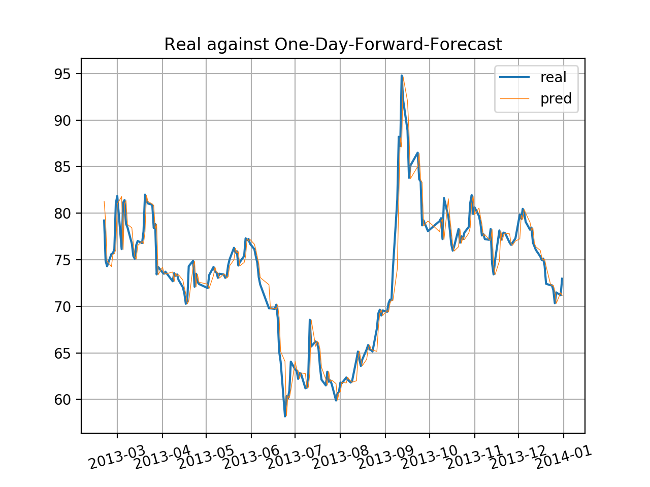
Finally, we perform out-of-sample test of ARIMA(1,0,0) by estimating one-day-forward price in each day of the sets with models built by the previous data. Continue the test every day beginning in the 100th index, and calculate the results. Because of limited space, we only provide a plot including the last 110 sets of predicted price against real price.

# Part VIII: Out-of-Sample Test for ARIMA(1,0,0) Performance
preds = []; lcs = []; ucs = []
for i in range(100,len(p_stk)):
    model_o = arima_model.ARIMA(p_stk[:i],order=(1,0,0)).fit()
    preds.append(model_o.forecast(1)[0][0])
    lcs.append(model_o.forecast(1)[2][0][0])
    ucs.append(model_o.forecast(1)[2][0][1])
plt.figure(dpi=200)
plt.grid(True)
plt.xticks(rotation=15)
plt.title('Real against One-Day-Forward-Forecast')
plt.plot(p_stk[1000:],ls='-')
dates = p_stk.index[1000:]
plt.plot(dates,preds[900:],lw=0.5)
plt.legend(['real','pred_ar1'])
plt.savefig('ARIMA_OStest.png')


By the way, we plot the errors of real minus estimated, and the result is very similar with the shape of returns. The errors might have patterns of heteroscedasticity, and perhaps one way to improve is to introduce ARCH or GARCH.

errors = p_stk[100:] - pd.Series(preds,index=p_stk.index[100:])
plt.figure(dpi=200)
plt.title('Errors of ARMA OS test')
plt.plot(errors)
plt.savefig('errors_of_ARIMA_OStest.png')

Reference:
Quantitative Investment Using Python, written by Lirui CAI, a Chinese Book named《量化投资:以Python为工具》

Tuesday, February 13, 2018

Feasible GLS (Generalized Least Squares)

GLS is applied when the residuals of OLS cannot satisfy two aspects of its classical assumptions: homoscedasticity and no auto-correlation, or rather,

$E(uu^{'})=\sigma ^{2}\Omega $

rather than

$E(uu^{'})=\sigma ^{2}I$

There are many forms of FGLS, and the following passage describes its basic theorem and one form of FGLS that could eliminate if there is only heteroscedasticity:

Theorem of GLS, WLS, and One Form of FGLS

There is also another model to eliminate only AR(1) pattern in the OLS residuals:

1) Estimate coefficient $\rho$ in the residuals that

$e_{t} = \rho e_{t-1} + \varepsilon$

2) Transfer

$y = X\beta +u $

to

$Py = PX\beta +Pu $

by


and 3) Estimate correspondingwith OLS estimation.

I will add more forms of FGLS in the following if possible.

Friday, February 2, 2018

Articles Related with Options Trading Strategies: Reading List

On Feb. 2018:

I.

Dubinsky A, Johannes M. Fundamental uncertainty, earning announcements and equity options[R]. Working paper, 2006.

Abstract:

This paper uses option prices to learn about the uncertainty surrounding the fundamental information that is revealed on earnings announcement dates. To do this, we introduce a reduced-form model and estimators to separate the uncertainty over the information revealed on earnings dates from normal day-to-day volatility. The fundamental uncertainty estimators are easy to compute and rely only on option price information available prior to the announcement. Empirically, we find strong support for our reduced form specification and investigate the fundamental uncertainty estimators. We find that they are quantitatively large, vary over time, and are informative about the future volatility of stock price movements. Finally, we quantify the impact of earnings announcements on formal option pricing models.

II.

Xing Y, Zhang X. Anticipating uncertainty: Straddles around earnings announcements[J]. 2013.

Abstract:

Straddles on individual stocks generally earn significantly negative returns. However, average at-the-money straddles from three days before an earnings announcement to the announcement date yield a highly significant 3.34% return. The positive returns on straddles indicate that investors under-estimate the magnitude of uncertainty around earnings announcements. We find positive straddle returns are more pronounced for smaller firms, firms with higher volatility, higher kurtosis, more volatile past earnings surprises and less trading volume/higher transaction costs. This
suggests that when firm signals are noisy, and/or when it is costlier to trade, investors underestimate the uncertainty associated with earnings announcements.

III.

Cremers M, Fodor A, Weinbaum D. How Do Informed Option Traders Trade? Option Trading Activity, News Releases, and Stock Return Predictability[J]. 2017.

Abstract:

We examine how informed traders trade in the option market around news announcements. Option traders are more active, and their trades more informative, both immediately before news days and on news days. How informed option traders implement their trades depends on when they trade and whether news releases are scheduled: we predict and find that informed option traders use short positions (instead of long positions) before scheduled news announcements. Purchases of options thus predict returns on news days and ahead of unscheduled events, but not before scheduled events, and sales of options are informative only ahead of scheduled news releases.

IV.

Jones C S, Shemesh J. Option Mispricing Around Nontrading Periods[J]. The Journal of Finance, 2017.

Abstract:

We find that option returns are significantly lower over nontrading periods, the vast majority of which are weekends. Our evidence suggests that nontrading returns cannot be explained by risk, but rather are the result of widespread and highly persistent option mispricing driven by the incorrect treatment of stock return variance during periods of market closure. The size of the effect implies that the broad spectrum of finance research involving option prices should account for nontrading effects. Our study further suggests how alternative industry practices could improve the efficiency of option markets in a meaningful way.