The results only include estimation of price, and backtest results like Sharpe are not calculated.
Firstly, we are doing some data preprocessing. The data 'SH50 Price.csv' includes the price information of the 50 listed in Shanghai Stock Exchange, components of SSE50 index, from 2009 to 2013. Data is available here.
# Data Preprocessing
import math
import pandas as pd
import numpy as np
from matplotlib import pyplot as plt
import ffn
df = pd.read_csv('SH50 Price.csv')
df.Date = pd.to_datetime(df.Date)
stocks = df.columns[1:].tolist()
prices = df[stocks]
prices.index = df.Date
simret = ffn.to_returns(df[stocks])
simret.index = df.Date
p_stk = prices['Stk_600000'][1:]
r_stk = simret['Stk_600000'][1:]
After preprocessing, we obtain price series 'p_stk' and returns series 'r_stk'. Then, we are going to have a glance at the information provided in the datasets. We choose stk 600000 as our target to research and forecast.
# Part I: Print figures
plt.figure(dpi=200)
plt.plot(p_stk)
plt.title('Price of Stk 600000')
plt.savefig('Price of Stk 600000.png')
plt.figure(dpi=200)
plt.plot(r_stk)
plt.title('Returns of Stk 600000')
plt.savefig('Returns of Stk 600000.png')
The plots are:


Because ARIMA requires that the time series should be stationary and not white noise, in the following two parts, we are using ADF Unitroot Test and Ljung-Box White Noise Test to evaluate the characteristics of the price and returns series.
# Part II: Test Stationary: ADF unitroot test
from arch.unitroot import ADF
adf = ADF(p_stk)
print(adf.summary()) #p-value: 0.042
adf = ADF(r_stk)
print(adf.summary()) #p-value: 0.000
Both of them are stationary, while returns series are more stationary as it has significantly smaller p-value, even though the p-value of prices are lower than 5%.
# Part III: Test White Noise: Ljung-Box test
from statsmodels.tsa import stattools
LjungBox_p = stattools.q_stat(stattools.acf(p_stk)[1:12],len(p_stk))
LjungBox_r = stattools.q_stat(stattools.acf(r_stk)[1:12],len(r_stk))
>> LjungBox_p
(array([ 1186.72403401, 2347.64336586, 3480.90920079, 4585.93740601,
5664.13867134, 6714.87739681, 7742.00626975, 8745.83186807,
9727.36536476, 10686.98822401, 11624.15953127, 12540.96124026,
13436.9868527 , 14312.56022102, 15168.03444284, 16003.30196641,
16817.86975455, 17612.10904286, 18385.5534396 , 19138.93560575,
19870.54594297, 20580.38199531, 21268.22774876]),
array([ 4.68328128e-260, 0.00000000e+000, 0.00000000e+000,
0.00000000e+000, 0.00000000e+000, 0.00000000e+000,
0.00000000e+000, 0.00000000e+000, 0.00000000e+000,
0.00000000e+000, 0.00000000e+000, 0.00000000e+000,
0.00000000e+000, 0.00000000e+000, 0.00000000e+000,
0.00000000e+000, 0.00000000e+000, 0.00000000e+000,
0.00000000e+000, 0.00000000e+000, 0.00000000e+000,
0.00000000e+000, 0.00000000e+000]))
>> LjungBox_r
(array([ 5.74442324e-05, 6.94963524e-01, 2.36008649e+00,
2.56248994e+00, 3.34789797e+00, 8.93787714e+00,
9.12876556e+00, 9.22065050e+00, 9.59020002e+00,
9.72752825e+00, 1.23203023e+01, 1.34820767e+01,
1.38328148e+01, 1.41616503e+01, 1.41655260e+01,
1.61315152e+01, 1.61315159e+01, 1.76274610e+01,
1.78485936e+01, 2.20053144e+01, 2.20102166e+01,
2.20334465e+01, 2.20547776e+01]),
array([ 0.99395273, 0.7064649 , 0.50110775, 0.63348204, 0.64651689,
0.17710208, 0.24354298, 0.32402559, 0.38466708, 0.46471465,
0.340055 , 0.3349957 , 0.38572255, 0.43773873, 0.51301413,
0.44382027, 0.51453146, 0.48043601, 0.5325723 , 0.34022234,
0.39892134, 0.45789384, 0.5169469 ]))
The null hypothesis is the series is white noise, and when the p-values (lower part of the result) of corresponding scores (upper part) are very small, we would reject the null hypothesis. In the prices, all values are highly significant, while the returns cannot reject the hypothesis (with 24 lags, the lowest one is even more then 10%).
Therefore, we accept that returns series are white noise, and we would only use price series in the following analysis.
# Part IV: Determine the order p and q in ARMA(p,q)
In part IV, we will use ARMA instead of ARIMA because we have already determined that order of I, d = 0 because returns are white noise. Next, we will determine the orders of ARMA(p,q).
Our first method to determine orders:
Draw ACF and PACF, and we found that ACF decays slowly while PACF suddenly drops, indicating an AR process only. We calculate its corresponding AIC and fit them with AR, setting maximum number of lags to be 12, and get the result that 1 is great. Check again with PACF plot, only lag 1 has significant coefficient. Therefore, we determine it to be AR(1) process.

axe1 = plt.subplot(211)
axe2 = plt.subplot(212)
plot1 = plot_acf(p_stk,lags=24,ax=axe1)
plot2 = plot_pacf(p_stk,lags=24,ax=axe2)
# Clear trend of AR only, with order for MA q = 0
# According to PACF, order p = 1
from statsmodels.tsa import ar_model
print(ar_model.AR(p_stk).select_order(maxlag=12,ic='aic')) # 1
Our alternative method to determine orders: Calculate the information criteria values of each order pairs.
order_determine = stattools.arma_order_select_ic(p_stk,ic=['bic','aic'])
>>order_determine
{'aic': 0 1 2
0 9463.164218 8000.817909 7042.006694
1 4518.521655 4520.130771 4520.321662
2 4520.100423 4520.516399 4521.249129
3 4520.254865 4521.373563 NaN
4 4520.303277 4520.282986 4517.939588,
'aic_min_order': (4, 2),
'bic': 0 1 2
0 9473.360970 8016.113036 7062.400197
1 4533.816782 4540.524274 4545.813540
2 4540.493925 4546.008277 4551.839383
3 4545.746743 4551.963817 NaN
4 4550.893531 4555.971616 4558.726593,
'bic_min_order': (1, 0)}
As BIC is more robust, the AIC of (1,0) is enarly the same with (4,2), and lower orders are better models to avoid overfitting risk, we choose ARMA(1,0), which leads to the same results with the above method.
# Part V: Fit prices with ARIMA(1,0,0) (Also ARMA(1,0) or AR(1))
# from statsmodels.tsa import ar_model
model = ar_model.AR(p_stk).fit(maxlag=12,method='cmle',ic='aic')
# arima_model package is a similar package, leading to a same result
from statsmodels.tsa import arima_model
model2 = arima_model.ARIMA(p_stk,order=(1,0,0)).fit()
Even though 'model' is the same with 'model2', the package ar_model has some bugs as I test it, and the package arima_model has attribute 'forecast' and it is more convenient to use this one. So, we only use model2 in the following parts.
>>model2.summary()

After ARMA modeling, we need to test whether the results of ARMA is white noise. If not, we may need more thorough researches. Fortunately, the results in the following shows that our result is white noise and no auto-correlation patterns.
# Part VI: Robustness Check: Test on Residuals
res = model2.resid
stdres = res/math.sqrt(model2.sigma2)
plt.figure(dpi=200)
ax1 = plt.subplot(211)
ax2 = plt.subplot(212)
ax1.set_title('standard residuals')
ax1.plot(stdres)
plot_acf(stdres,lags=24,ax=ax2)
plt.savefig('test_on_residuals_of_ARMA.png')

LjungBox_m = stattools.q_stat(stattools.acf(stdres[1:])[1:24],len(stdres[1:]))
# Residuals are White Noises
>>LjungBox_m
(array([ 0.27569431, 1.76892747, 3.40736876, 4.00228122,
4.30689222, 8.74894778, 8.75161177, 8.79754988,
8.84251288, 9.8780216 , 12.49860582, 13.03671273,
13.05266838, 13.31819495, 13.83520634, 16.51855888,
16.83245856, 18.33579538, 18.40466682, 23.02723339,
23.05146308, 23.051464 , 23.17217018]),
array([ 0.59953731, 0.41293556, 0.33297629, 0.40569721, 0.50612843,
0.18819711, 0.27098469, 0.35966135, 0.45193696, 0.45125936,
0.32735392, 0.3663779 , 0.44375169, 0.50163586, 0.53806246,
0.41739165, 0.46577191, 0.43374623, 0.49557738, 0.2874593 ,
0.34124064, 0.39882846, 0.45075531]))
To conclude, we cannot reject that results white noise, and the ARMA models can be used to forecast.
In the next part, we are going to give a forward forecast on the results, and plot corresponding confidence intervals.
# Part VII: Forecast
forecast = model2.forecast(steps=15)
plt.figure(dpi=200)
plt.grid(True)
plt.xticks(rotation=15)
plt.title('ARIMA(1,0,0) Forecast for Stk 600000')
plt.plot(p_stk[-30:])
dates = pd.DatetimeIndex(freq='d',start='2014-01-01',end='2014-01-15')
plt.plot(dates,forecast[0])
plt.plot(dates,forecast[2][:,0],ls=':')
plt.plot(dates,forecast[2][:,1],ls=':')
plt.legend(['real','pred','lc','uc'])
plt.savefig('ARIMA_forecast.png')

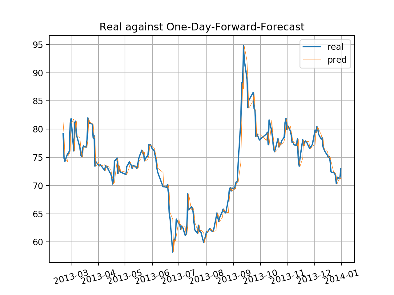
Finally, we perform out-of-sample test of ARIMA(1,0,0) by estimating one-day-forward price in each day of the sets with models built by the previous data. Continue the test every day beginning in the 100th index, and calculate the results. Because of limited space, we only provide a plot including the last 110 sets of predicted price against real price.
# Part VIII: Out-of-Sample Test for ARIMA(1,0,0) Performance
preds = []; lcs = []; ucs = []
for i in range(100,len(p_stk)):
model_o = arima_model.ARIMA(p_stk[:i],order=(1,0,0)).fit()
preds.append(model_o.forecast(1)[0][0])
lcs.append(model_o.forecast(1)[2][0][0])
ucs.append(model_o.forecast(1)[2][0][1])
plt.figure(dpi=200)
plt.grid(True)
plt.xticks(rotation=15)
plt.title('Real against One-Day-Forward-Forecast')
plt.plot(p_stk[1000:],ls='-')
dates = p_stk.index[1000:]
plt.plot(dates,preds[900:],lw=0.5)
plt.legend(['real','pred_ar1'])
plt.savefig('ARIMA_OStest.png')
By the way, we plot the errors of real minus estimated, and the result is very similar with the shape of returns. The errors might have patterns of heteroscedasticity, and perhaps one way to improve is to introduce ARCH or GARCH.
errors = p_stk[100:] - pd.Series(preds,index=p_stk.index[100:])
plt.figure(dpi=200)
plt.title('Errors of ARMA OS test')
plt.plot(errors)
plt.savefig('errors_of_ARIMA_OStest.png')

Reference:
Quantitative Investment Using Python, written by Lirui CAI, a Chinese Book named《量化投资:以Python为工具》
No comments:
Post a Comment